R で負の二項回帰モデルを実行する方法

負の二項回帰モデルを R で行う方法

負の二項モデルを R で行う方法

まず、データを読み込む

X <- c(rep(1, 913), rep(2, 1345), rep(3, 519), rep(9, 863))
Y <- c(rep(0, 910), rep(1, 2), rep(2, 1), rep(4, 0),
rep(0, 1333), rep(1, 11), rep(2, 1), rep(4, 0),
rep(0, 509), rep(1, 9), rep(2, 1), rep(4, 0),
rep(0, 849), rep(1, 13), rep(2, 0), rep(4, 1))
dat <- data.frame(X, Y)

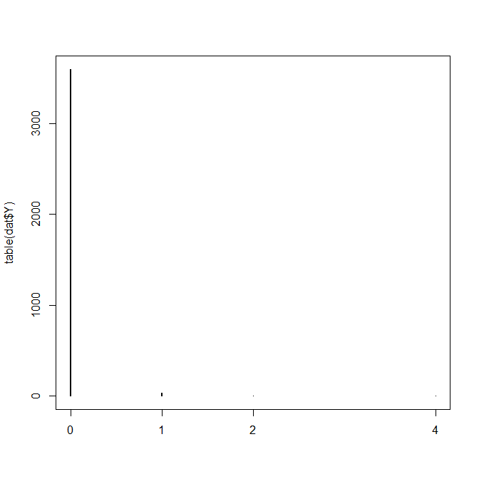
Yの分布を確認

> table(dat$Y)
   0    1    2    4
3601   35    3    1

Yの分布図はすごいことに、なっている

plot(table(dat$Y))

XとYの関係を見ていこう

まずクロス集計表

> table(dat$X, dat$Y)
     0    1    2    4
1  910    2    1    0
2 1333   11    1    0
3  509    9    1    0
9  849   13    0    1

Y がゼロばかりなのが目立つ

負の二項回帰モデルは、MASS パッケージの glm.nb() を使う

library(MASS)
nb.res <- glm.nb(Y ~ factor(X), data=dat)
summary(nb.res)

結果は、Xが１に比べて、３とか、９とかはYに関連がある

> summary(nb.res)
Call:
glm.nb(formula = Y ~ factor(X), data = dat, init.theta = 0.05009536409,
link = log)
Deviance Residuals:
Min        1Q    Median        3Q       Max
-0.18802  -0.18228  -0.13295  -0.09165   3.10151
Coefficients:
Estimate Std. Error z value Pr(>|z|)
(Intercept)  -5.4304     0.5214 -10.415   <2e-16 ***
factor(X)2    0.7912     0.6030   1.312   0.1895
factor(X)3    1.5764     0.6334   2.489   0.0128 *
factor(X)9    1.5032     0.5948   2.527   0.0115 *
---
Signif. codes:  0 ‘***’ 0.001 ‘**’ 0.01 ‘*’ 0.05 ‘.’ 0.1 ‘ ’ 1
(Dispersion parameter for Negative Binomial(0.0501) family taken to be 1)
Null deviance: 210.18  on 3639  degrees of freedom
Residual deviance: 199.65  on 3636  degrees of freedom
AIC: 465.67
Number of Fisher Scoring iterations: 1
Theta:  0.0501
Std. Err.:  0.0236
2 x log-likelihood:  -455.6660

まとめ

負の二項回帰モデルを R で実行する方法を簡単に紹介した

MASS パッケージの glm.nb() 関数を使うと実行できる